Using an AI desktop agent can handle data engineering steps so you can get straight to analysis.
Open geospatial data is more accessible than ever, but “accessible” doesn’t always mean “ready to use.” Large datasets frequently arrive as chunked, compressed files that need to be inventoried, understood, and consolidated before they can be loaded into a GIS. That’s exactly the kind of repetitive, multi-step data wrangling that Claude Cowork was built for.
This post walks through a short workflow that takes US railroad line data from the HIFLD Open archive on Source Cooperative — five compressed GeoJSON chunks — and turns it into a single, analysis-ready GeoParquet file that opens directly in QGIS 4.0.
Step 1: Locate the Source Data
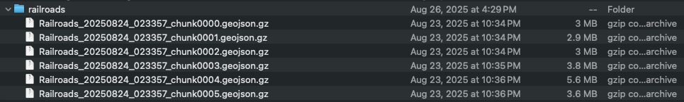
After downloading, the starting point is a folder called railroads, containing five GeoJSON files compressed as .gz archives — chunk0000 through chunk0004 — ranging from roughly 3 to 6 MB each. This is a typical delivery format for large vector datasets from Source Cooperative, where data is partitioned into manageable chunks for efficient downloading.
At this stage the data is opaque. You know what it’s called, but not what’s inside, how it’s structured, or whether it’s ready to use. Before touching any GIS tool, it’s worth understanding what you actually have. This is where we open Claude Cowork and get to work.
Step 2: Ask Claude to Summarize the Dataset
Rather than manually decompressing and inspecting each file, the user simply asks Claude to summarize the folder contents. Within seconds, Claude reads through the chunked files and returns a concise description: the dataset contains US railroad lines (RRTE feature class), stored as MULTILINESTRING geometries in NAD-83 decimal degrees, with metadata embedded and the full dataset spanning the contiguous United States.
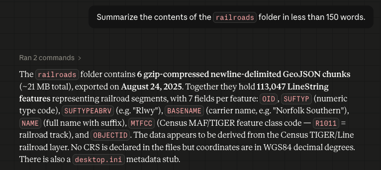
This step matters more than it might seem. Knowing the geometry type, CRS, and feature class upfront means no surprises when you go to load or reproject the data — and it takes about ten seconds.
Step 3: Merge All Chunks into a Single GeoParquet File
With the dataset understood, the next step is consolidation. The user gives Claude a single instruction: merge all five chunks into one GeoParquet file. What follows is a small but complete autonomous workflow.
Claude first determines what Python libraries it needs — geopandas to read the compressed GeoJSON files and write GeoParquet, pyarrow as the required columnar backend, and pyogrio for faster file I/O. Since these aren’t available in the base environment, it creates a virtual environment, installs the dependencies via pip, and then writes a Python script that globs all .geojson.gz files in the folder, reads each one into a GeoDataFrame, concatenates them, confirms the CRS is set to EPSG:4326, and calls to_parquet() to write the output. It then executes the script and verifies the result by reading the file back and printing a summary.
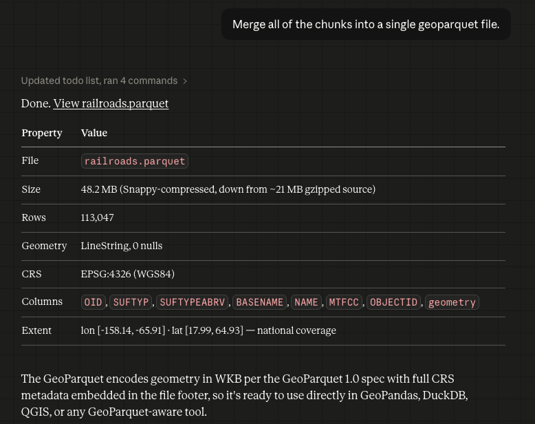
The result is a single .geoparquet file (~2 MB, gzip-compressed) with geometry type MULTILINESTRING, CRS confirmed as EPSG:4326 (WGS84), and the bounding box spanning the contiguous United States. Full CRS metadata is embedded in the file itself — no sidecar files, no manual projection setup. GeoParquet is an ideal target format for exactly this reason: it’s compact, column-oriented, and natively supported by GeoPandas, DuckDB — and as of QGIS 4.0, directly in the desktop GIS itself, with no intermediate conversion required.
It’s worth noting that all of the above processing happened in the background. By the time we are viewing the geoparquet file in Finder, the python venv has been been completely torn down and deleted.
Step 4: Visualize the Result in QGIS 4.0
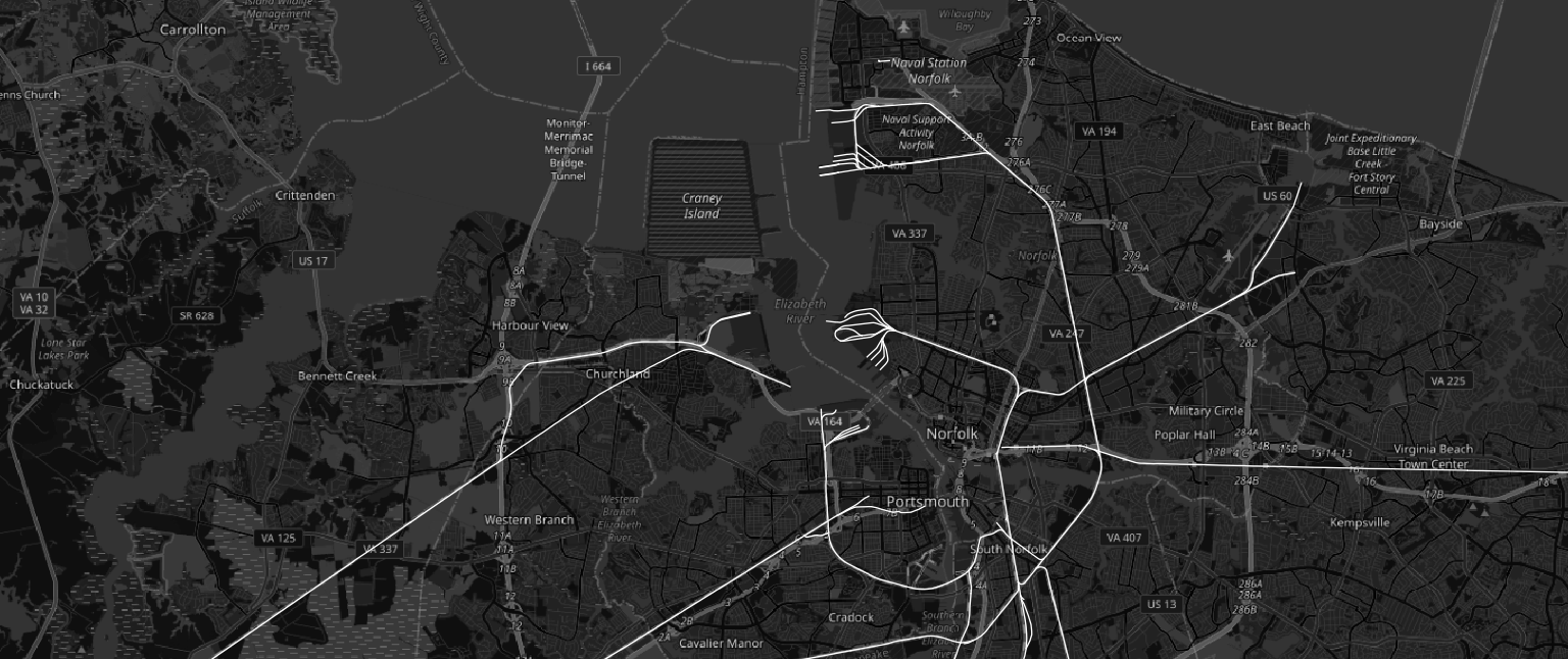
The merged GeoParquet file loads directly into QGIS 4.0 without any additional processing. Rendered against a dark basemap, the US railroad network comes into immediate focus — dense corridors in the eastern half of the country, clear transcontinental routes running west, and the unmistakable shape of a century-plus of infrastructure investment.
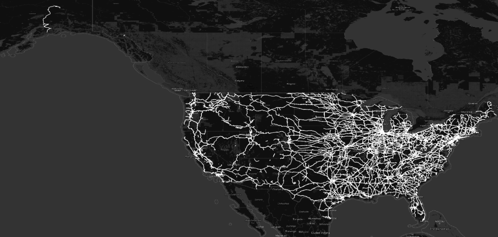
The map is a confirmation as much as a visualization: the data is clean, the geometry is valid, the projection is correct, and the full national extent is present. Everything worked.
What This Workflow Means
The four steps above took a few minutes. Without an AI assistant, the same process of locating and auditing chunked files, writing a merge script, handling CRS differences, and outputting to the right format could easily take an hour, especially if you’re working across unfamiliar data sources.
Claude Cowork handles the data engineering layer: reading, interpreting, transforming, and validating. The GIS practitioner stays focused on the geographic question they actually want to answer.
The HIFLD Open archive on Source Cooperative is a rich source of authoritative US infrastructure data. Pair it with a capable AI assistant and a modern GIS desktop, and the path from raw download to ready-to-analyze layer is shorter than it’s ever been.
The term “GeoAI” can mean a lot of things, but it doesn’t have to mean releasing your entire production workflow to AI. Tools such as Claude Cowork are making targeted AI workflows more accessible to knowledge workers without the need for writing additional code. They provide a means to streamline rote tasks while enabling analysts to focus their expertise on core problems.